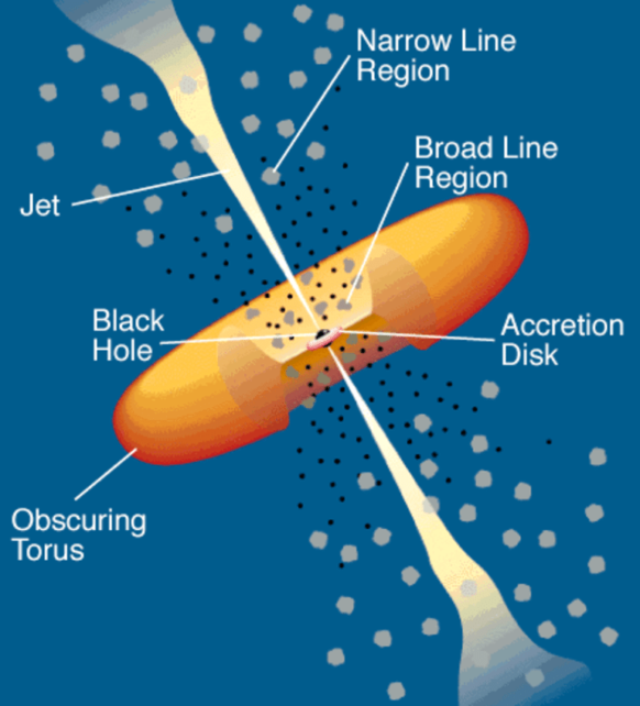
A year into my research and I’m slowly uncovering a lot about the zoo that populates objects under the title “Active Galactic Nuclei” (AGN). The fact that they are multi-wavelength emitters means that we get a variety of features to try and understand across different energy bands, but that also means that categories and sub-categories have become increasingly complex to describe them. The most straightforward standard model includes the central black hole, an accretion disk, a jet, an obscuring torus, and ionized clouds of gas near the black hole (broad/narrow line region; AGN model shown in Figure 1). Around the 1990s, a unification scheme for the numerous features of AGN was proposed by Antonucci 1993; Urry & Padovani 1995 which depended primarily on inclination, accretion rate, and the appearance of a jet. For my work, inclination is (almost) everything.
For some context, I’m studying a sample of sources that have all been denoted “low-luminosity active galactic nuclei” (LLAGN) which physically means that their luminosity is < 10^43 erg s-1. While we define them as low-luminosity, it’s really the rate of accretion by the supermassive black hole at the center that we’re concerned with. These LLAGN are assume to be accreting material at efficiencies η = 10-9 – 10-3 MEdd, where MEdd is the Eddington scaled accretion rate, defined with LEdd = 1.26 * 1038(MBH/MSun) erg s-1, and LEdd = η MEdd c2. This low accretion rate is assumed to change the structure of the flow of material around the black hole, where it transitions from the standard thin disk (Shakura & Sunyaev, 1973) to a thicker, puffy disk (radiatively inefficient accretion flow; see reviews by Narayan et al. 1998, Quataert 2001). They’re also our most popular galactic neighbor, which means that they could represent an important stage in the lives of AGN systems. For my work, I’m interested in pinning down some of their continuum properties: dominant emission mechanisms for the inner + outer regions, how similar they behave from source to source, and what correlation their behavior might have with things like central black hole mass or accretion rate. This involves studying the multi-wavelength spectrum from these objects, which I compare to a multi-zone leptonic jet model, initially written by Sera Markoff (Markoff et al. 2000) and then developed by a former group member, Matteo Lucchini (Github: BHJet; Lucchini et al. 2022).
As the name suggests, these objects are low luminosity: the nuclear region may not be very bright, but the surrounding galaxy still can be. Therefore, it can be quite difficult to disentangle the processes taking place near the nuclear region from the brighter nearby emission that can easily outshine it. One way to counter this is to use high-angular resolution observations to ensure that when we focus on the nuclear region, we can try to minimize contributions from the host galaxy. However, if we go back to the overview of AGN components I listed above, you’ll note the word “obscuring” in front of “torus”. This torus is assumed to be a clumpy region of dust, located at the outer edges of the accretion disk. Emission from the central region that travels through the torus can be subject to intensive absorption and reprocessing, based on the density of material within the torus. Therefore, depending on the inclination and makeup of the torus for a given AGN, it can shroud the emission from inner regions, making it even more difficult to decipher what AGN and LLAGN are up to.
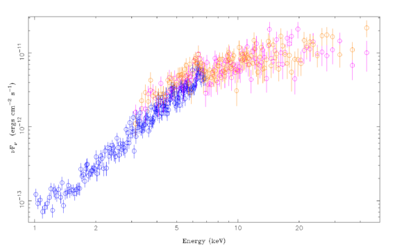
So, as I got further into studying the multi-wavelength emission from my sources, I started to realize that something was “up” with the X-ray emission. If we have a clear line of sight to the AGN, and we point an X-ray telescope at it, we typically assume that this emission, or the nuclear X-ray continuum, can be described by a power law with an index between Γ= 1.4 and 2.1. However, when I started reducing X-ray data of my sources, I was finding that some of my spectra had a variety of features, and the overall shape was not specifically reminiscent of a power-law. Figure 1 shows an “unfolded” X-ray spectrum for NGC 1052, with observations taken from the Chandra (blue) and NuSTAR (orange, pink) telescopes. For starters, at lower energies (1 – 7 keV), I had a strong dip in the Chandra part of the spectrum. However, the smoking gun that tells us something else is going on sits at 6.4 keV: the Fe K alpha emission line. The appearance of this line in the X-ray spectrum tells us that the X-rays are reflecting off some material in the system, and in this case, the material in the obscuring torus.
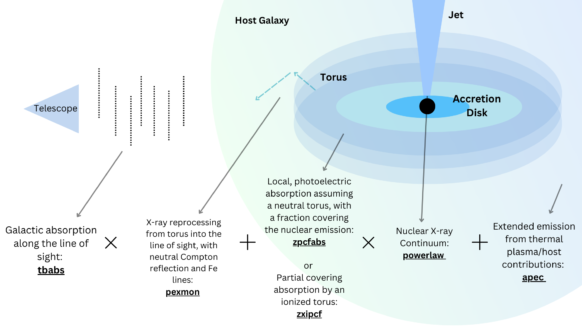
So, in order to try and uncover what my low-luminosity AGN are up to, I need to make sure I can accurately describe all the additional processes that are impacting the nuclear emission, if I want to obtain the underlying spectrum. Figure 2 shows a (not to scale) toy figure for some of the different spectral models that can be applied to the spectrum in order to try and describe the properties of the region. So, for each source in my sample, I can use the inclination angle of the jet as well as study the features of the X-rays to try and make some predictions on what I’ll need to do to uncover the underlying spectrum at these energies. Further, when I go to apply BHJet to the full spectrum, it’s important that I have a good description of what is going on in the X-rays.
The punchline of this post is that I’ve learned so many things that I hardly anticipated to when I started this project, from reducing and using X-ray data, to jointly modeling many observations together to try and infer properties of both the medium and the nuclear emission, to fighting with my spectral analysis software and get it to cooperate with me. (And don’t even get me started about the Optical/UV regions). For the larger context of my project, it’s really helped me to think about what is taking place in and around these central regions in AGN and how I interpret the results that I find. There is still much to figure out, of course!